How We Managed to Reduce SQS Costs and Pricing by 90%

Reading Time: 5 minutes

Our SDKs help our customers track click-stream data along with the user attributes. The data is then sent to the MoEngage servers for further processing. However, due to its voluminous nature, the data needs to be optimized, which is achieved by batching the data before it hits our servers. As the traffic(rpm) to our servers isn’t predictable, we first put the data in the AWS SQS to handle any unusual spikes and later process it at the rate which our server can handle.

Premise

Moving the data to SQS before it hits the server directly is good practice, though, the following areas needed improvement:

1. Latency: Though SQS response times are the best in the industry, every API call from the SDK adds to the overall response time – increasing the latency.
2. Costs: SQS pricing is based on the no. of messages that are put in the queue, deleted from the queue, and consumed from the queue. So, every message would be billed thrice. Given the scale at we are operating, SQS processing with no intelligence layer made little business sense.

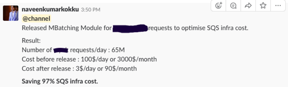
In the picture below, you can see one of our team members posting the improvements we saw after enabling the solution for one of the clients

Solution

The obvious solution to this problem is to batch the data before sending to the SQS, but this comes with inherent challenges –

1. How many requests do we batch and how would it affect the latency perceived by the customer? Latency is defined as the time taken for the SDK to track the data and display it to the marketer on the dashboard.
2. SQS has a cap on each message size to be less than 256KB, and anything more than that, it throws an exception. Average message size in our case is 5KB. If a message size exceeds 64KB, each 64KB chunk is treated as a separate message for billing.

We’ve addressed these issues by defining a few rules, and finally, arrived at a concrete solution (MBatching) in which:

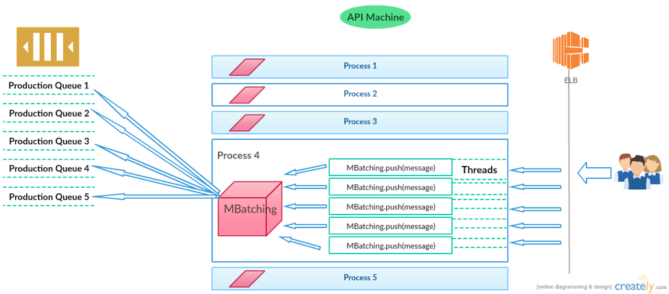
1. Each API server would have a MBatching module to interact with SQS.
2. Store each message in the local queue, and when the compressed size of the messages reaches close to 64KB, compress the existing messages into a single message and flush it to SQS.
3. A cap on the flush time – Sometimes, it may take more time to reach 64KB size cap. So, each service that is leveraging MBatching is given a configurable parameter to flush the messages based on time.

In the picture below, we have explained how MBatching fits into our architecture –

MBatching module has an additional requirement to meet – The solution has to be generic so that we can work with multiple queues on SQS from a single machine.

Anything we build at MoEngage, we try to make it versatile to suit most of our needs across the company.

Design

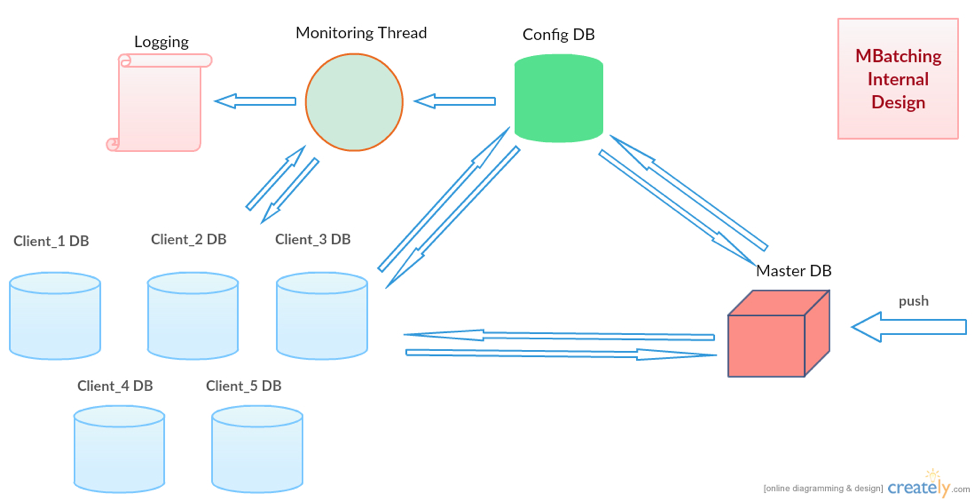
MBatching internally has four key components:

1. MasterDB – Data store which separately stores the messages for each service.
2. ConfigDB – Data store for every process on the machine, that stores the local queues availability status and keeps references to the local queue of each service.
3. Monitor – Thread to validate the number of messages received and processed. The key functionality of this thread is to validate data loss and raise alerts if any.
4. Analyser – Thread which evaluates the optimum number of messages that can be compressed before sending to SQS.

Internal design overview of MBatching is mentioned in the picture below –

Lifecycle of a message

Let’s look at the lifecycle of a message, to understand how all the components work together.

When a message is received at the MBatching module, it first checks if a local queue exists, if not, a queue is created, let’s call this localQ. A counter is maintained to keep track of the no.of messages received in the localQ, and it is incremented accordingly. Next, we check the size of the sum of uncompressed messages in localQ and whether it exceeds a threshold value – 80KB (we have tuned and arrived at this value from our experiments). If it does exceed the threshold, we flush all the messages to another queue, call it mergeQ. Similar to localQ, a counter is maintained to keep track of how many messages are sent to mergeQ and this counter is incremented accordingly. Parallely, the analyzer works on mergeQ in a separate thread to find out the optimum number of messages required to reach the 64KB compressed size. We will discuss the need for two queues after we explain how compression works.

Analyser is responsible to compress the messages in mergeQ and send them to SQS. This is how analyser works –

1. Calculate the compression size of all the message in mergeQ, if it’s greater than 50KB (tuned from experiments) and less than 64KB, send them to SQS.
2. If the compression size is less than 50KB, do nothing.
3. If the compression size is more than 64KB –
   1. Sort the messages in ascending order by size.
   2. Pick the first half of messages and check the compression size, if not optimal, add the first half of the second half and go on until, we find the optimal size. (Merge sort concepts used here)
   3. Compress and flush the optimal messages to SQS.
   4. Let the remaining messages lie in mergeQ.

A message at a given point of time, will reside in localQ or mergeQ, before it eventually gets flushed to SQS.

If we were to do the compression logic in localQ, first we would have to lock the queue. And then all the API requests would be waiting on this queue to become free to put the messages in it until the compression logic is computed. Hence, to optimize the performance, the analyser is initiated in a separate thread, where only 1 API call is taking the load of evaluating compression logic.

Each service can also mention the max time to wait to achieve optimal compression. Monitor thread uses this time to validate data loss periodically, triggered every x mins.

Here is how monitoring thread works –

1. Find out all the localQ information, which is stored in configDB.
2. Flush all the messages in localQ to mergeQ, and mergeQ is also flushed optimally, except for the remaining last half if any.
3. Validate the counters for localQ, if the no.of messages received and no.of messages sent to mergeQ are equal. Raise an alert if there is any mismatch.

Impact

We were able to reduce our SQS costs by a whopping 90%. Better yet, the response time for MBatching module is 1ms compared to 10ms contacting SQS.

Thanks to our innovative engineering team, we have been using MBatching in production for almost two years now, and it has worked wonders for us.

If you like working on challenging problems at scale and solve them optimally, we would like for you to be part of our team, please check the job openings here.

Say Hi on Twitter or check out what we’re building at MoEngage